CL 2- C2 Tizen programming

Official Developer website of Tizen

Naive Bayes algorithm

Table of Contents

1. What is Naive Bayes algorithm?
2. How Naive Bayes Algorithms works?
3. What are the Pros and Cons of using Naive Bayes?
4. 4 Applications of Naive Bayes Algorithm
5. Steps to build a basic Naive Bayes Model in Python
6. Tips to improve the power of Naive Bayes Model

What is Naive Bayes algorithm?

It is a classification technique based on Bayes’ Theorem with an assumption of independence among predictors. In simple terms, a Naive Bayes classifier assumes that the presence of a particular feature in a class is unrelated to the presence of any other feature. For example, a fruit may be considered to be an apple if it is red, round, and about 3 inches in diameter. Even if these features depend on each other or upon the existence of the other features, all of these properties independently contribute to the probability that this fruit is an apple and that is why it is known as ‘Naive’.

Naive Bayes model is easy to build and particularly useful for very large data sets. Along with simplicity, Naive Bayes is known to outperform even highly sophisticated classification methods.

Bayes theorem provides a way of calculating posterior probability P(c|x) from P(c), P(x) and P(x|c). Look at the equation below:

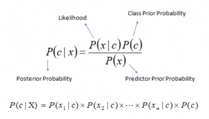Above,

• P(c|x) is the posterior probability of class (c, target) given predictor (x, attributes).
• P(c) is the prior probability of class.
• P(x|c) is the likelihood which is the probability of predictor given class.
• P(x) is the prior probability of predictor.

How Naive Bayes algorithm works?

Let’s understand it using an example. Below I have a training data set of weather and corresponding target variable ‘Play’ (suggesting possibilities of playing). Now, we need to classify whether players will play or not based on weather condition. Let’s follow the below steps to perform it.

Step 1: Convert the data set into a frequency table

Step 2: Create Likelihood table by finding the probabilities like Overcast probability = 0.29 and probability of playing is 0.64.

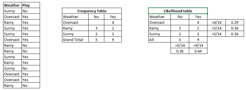
Step 3: Now, use Naive Bayesian equation to calculate the posterior probability for each class. The class with the highest posterior probability is the outcome of prediction.

Problem: Players will play if weather is sunny. Is this statement is correct?

We can solve it using above discussed method of posterior probability.

P(Yes | Sunny) = P( Sunny | Yes) * P(Yes) / P (Sunny)

Here we have P (Sunny |Yes) = 3/9 = 0.33, P(Sunny) = 5/14 = 0.36, P( Yes)= 9/14 = 0.64

Now, P (Yes | Sunny) = 0.33 * 0.64 / 0.36 = 0.60, which has higher probability.

Naive Bayes uses a similar method to predict the probability of different class based on various attributes. This algorithm is mostly used in text classification and with problems having multiple classes.

What are the Pros and Cons of Naive Bayes?

Pros:

• It is easy and fast to predict class of test data set. It also perform well in multi class prediction
• When assumption of independence holds, a Naive Bayes classifier performs better compare to other models like logistic regression and you need less training data.
• It perform well in case of categorical input variables compared to numerical variable(s). For numerical variable, normal distribution is assumed (bell curve, which is a strong assumption).

Cons:

• If categorical variable has a category (in test data set), which was not observed in training data set, then model will assign a 0 (zero) probability and will be unable to make a prediction. This is often known as “Zero Frequency”. To solve this, we can use the smoothing technique. One of the simplest smoothing techniques is called Laplace estimation.
• On the other side naive Bayes is also known as a bad estimator, so the probability outputs frompredict_proba are not to be taken too seriously.
• Another limitation of Naive Bayes is the assumption of independent predictors. In real life, it is almost impossible that we get a set of predictors which are completely independent.

4 Applications of Naive Bayes Algorithms

• Real time Prediction: Naive Bayes is an eager learning classifier and it is sure fast. Thus, it could be used for making predictions in real time.
• Multi class Prediction: This algorithm is also well known for multi class prediction feature. Here we can predict the probability of multiple classes of target variable.
• Text classification/ Spam Filtering/ Sentiment Analysis: Naive Bayes classifiers mostly used in text classification (due to better result in multi class problems and independence rule) have higher success rate as compared to other algorithms. As a result, it is widely used in Spam filtering (identify spam e-mail) and Sentiment Analysis (in social media analysis, to identify positive and negative customer sentiments)
• Recommendation System: Naive Bayes Classifier and Collaborative Filtering together builds a Recommendation System that uses machine learning and data mining techniques to filter unseen information and predict whether a user would like a given resource or not

How to build a basic model using Naive Bayes in Python?

Again, scikit learn (python library) will help here to build a Naive Bayes model in Python. There are three types of Naive Bayes model under scikit learn library:

• Gaussian: It is used in classification and it assumes that features follow a normal distribution.
• Multinomial: It is used for discrete counts. For example, let’s say,  we have a text classification problem. Here we can consider bernoulli trials which is one step further and instead of “word occurring in the document”, we have “count how often word occurs in the document”, you can think of it as “number of times outcome number x_i is observed over the n trials”.
• Bernoulli: The binomial model is useful if your feature vectors are binary (i.e. zeros and ones). One application would be text classification with ‘bag of words’ model where the 1s & 0s are “word occurs in the document” and “word does not occur in the document” respectively.

Based on your data set, you can choose any of above discussed model. Below is the example of Gaussian model.

Python Code

#Import Library of Gaussian Naive Bayes model
from sklearn.naive_bayes import GaussianNB
import numpy as np

#assigning predictor and target variables
x= np.array([[-3,7],[1,5], [1,2], [-2,0], [2,3], [-4,0], [-1,1], [1,1], [-2,2], [2,7], [-4,1], [-2,7]])
Y = np.array([3, 3, 3, 3, 4, 3, 3, 4, 3, 4, 4, 4])

#Create a Gaussian Classifier
model = GaussianNB()

# Train the model using the training sets 
model.fit(x, y)

#Predict Output 
predicted= model.predict([[1,2],[3,4]])
print predicted

Output: ([3,4])

Above, we looked at the basic Naive Bayes model, you can improve the power of this basic model by tuning parameters and handle assumption intelligently. Let’s look at the methods to improve the performance of Naive Bayes Model. I’d recommend you to go through this document for more details on Text classification using Naive Bayes.

Tips to improve the power of Naive Bayes Model

Here are some tips for improving power of Naive Bayes Model:

• If continuous features do not have normal distribution, we should use transformation or different methods to convert it in normal distribution.
• If test data set has zero frequency issue, apply smoothing techniques “Laplace Correction” to predict the class of test data set.
• Remove correlated features, as the highly correlated features are voted twice in the model and it can lead to over inflating importance.
• Naive Bayes classifiers has limited options for parameter tuning like alpha=1 for smoothing, fit_prior=[True|False] to learn class prior probabilities or not and some other options (look at detail here). I would recommend to focus on your  pre-processing of data and the feature selection.
• You might think to apply some classifier combination technique like ensembling, bagging and boosting but these methods would not help. Actually, “ensembling, boosting, bagging” won’t help since their purpose is to reduce variance. Naive Bayes has no variance to minimize.

Unification algorithm with examples

Unification is essentially a process of substitution. I have seen it called "two-way matching". In Prolog, in other logic programming languages and in languages directly based on rewriting logic (Maude, Elan, etc...) is the mechanism by which free (logical) variables are bind to terms/values. In Concurrent Prolog these variables are interpreted as communication channels. IMO, the better way to understand it is with some examples from mathematics (unification was/is a base key mechanism, for example, in the context of automated theorem provers research, a sub-field of AI; another use in in type inference algorithms). The examples that follow are taken from the context of computer algebra systems (CAS): First example: given a set Q and two binary operations * and + on it, then * is left-distributive over + if: X * (Y + Z)   =   (X * Y) + (X * Z)   |1| this is a rewrite rule (a set of rewrite rules is a rewriting system). If we want to apply this rewrite rule to a specific case, say: a * (1 + b)   |2| we unify (via a unification algorithm) this term, |2|, with the left-hand side (lhs) of |1| and we have this (trivial on purpose) substitution (the most general unifier, mgu): {X/a, Y/1, Z/b}   |3| Now, applying |3| to the right-hand side (rhs) of |1|, we have, finally: (a * 1) + (a * b) This was simple and to appreciate what unification can do I will show a little more complex example. Second example: Given this rewrite rule: log(X,Y) + log(X,Z)   =>   log(X,Y*Z)   |4| we apply it to this equation: log(e,(x+1)) + log(e,(x-1)) = k   |5| (lhs of |5| unify to lhs of |4|), so we have this mgu: {X/e, Y/(x+1), Z/(x-1)}   |6| Note that X and x are two different variables. Here we have two variables, X and Y, which match two compound terms, (x+1) and (x-1), not simple values or variables. We apply this mgu, |6|, to rhs of |4| then and we put back this in |5|; so we have: log(e,(x+1)*(x-1)) = k   |7| and so on.

Applications of uninformed search methods : Depth First Search

In this article, applications of Depth  First Search are discussed.

1) For an unweighted graph, DFS traversal of the graph produces the minimum spanning tree and all pair shortest path tree.

2) Detecting cycle in a graph 
A graph has cycle if and only if we see a back edge during DFS. So we can run DFS for the graph and check for back edges. (See this for details)

3) Path Finding
We can specialize the DFS algorithm to find a path between two given vertices u and z.
i) Call DFS(G, u) with u as the start vertex.
ii) Use a stack S to keep track of the path between the start vertex and the current vertex.
iii) As soon as destination vertex z is encountered, return the path as the
contents of the stack

See this for details.

4) Topological Sorting
Topological Sorting is mainly used for scheduling jobs from the given dependencies among jobs. In computer science, applications of this type arise in instruction scheduling, ordering of formula cell evaluation when recomputing formula values in spreadsheets, logic synthesis, determining the order of compilation tasks to perform in makefiles, data serialization, and resolving symbol dependencies in linkers [2].

5) To test if a graph is bipartite
We can augment either BFS or DFS when we first discover a new vertex, color it opposited its parents, and for each other edge, check it doesn’t link two vertices of the same color. The first vertex in any connected component can be red or black! See this for details.

6) Finding Strongly Connected Components of a graph A directed graph is called strongly connected if there is a path from each vertex in the graph to every other vertex. (See this for DFS based algo for finding Strongly Connected Components)

7) Solving puzzles with only one solution, such as mazes. (DFS can be adapted to find all solutions to a maze by only including nodes on the current path in the visited set.)

Applications of uninformed search methods :Breadth First Search

In this article, applications of Breadth First Search are discussed.

1) Shortest Path and Minimum Spanning Tree for unweighted graph In unweighted graph, the shortest path is the path with least number of edges. With Breadth First, we always reach a vertex from given source using minimum number of edges. Also, in case of unweighted graphs, any spanning tree is Minimum Spanning Tree and we can use either Depth or Breadth first traversal for finding a spanning tree.

2) Peer to Peer Networks. In Peer to Peer Networks like BitTorrent, Breadth First Search is used to find all neighbor nodes.

3) Crawlers in Search Engines: Crawlers build index using Breadth First. The idea is to start from source page and follow all links from source and keep doing same. Depth First Traversal can also be used for crawlers, but the advantage with Breadth First Traversal is, depth or levels of built tree can be limited.

4) Social Networking Websites: In social networks, we can find people within a given distance ‘k’ from a person using Breadth First Search till ‘k’ levels.

5) GPS Navigation systems: Breadth First Search is used to find all neighboring locations.

6) Broadcasting in Network: In networks, a broadcasted packet follows Breadth First Search to reach all nodes.

7) In Garbage Collection: Breadth First Search is used in copying garbage collection using Cheney’s algorithm. Refer this and for details. Breadth First Search is preferred over Depth First Search because of better locality of reference:

8) Cycle detection in undirected graph: In undirected graphs, either Breadth First Search or Depth First Search can be used to detect cycle. In directed graph, only depth first search can be used.

9) Ford–Fulkerson algorithm In Ford-Fulkerson algorithm, we can either use Breadth First or Depth First Traversal to find the maximum flow. Breadth First Traversal is preferred as it reduces worst case time complexity to O(VE2).

10) To test if a graph is Bipartite We can either use Breadth First or Depth First Traversal.

11) Path Finding We can either use Breadth First or Depth First Traversal to find if there is a path between two vertices.

12) Finding all nodes within one connected component: We can either use Breadth First or Depth First Traversal to find all nodes reachable from a given node.

Many algorithms like Prim’s Minimum Spanning Tree and Dijkstra’s Single Source Shortest Path use structure similar to Breadth First Search.

There can be many more applications as Breadth First Search is one of the core algorithm for Graphs

AI PR. based theory-2

In part1 we have introduced the problem formulation and how we judge on a certain search strategy, This article covers 5 uniformed search strategies in which all we know about the problem is its definition and no additional information about its states beyond those told in the problem definition.

Uniformed search strategies are very systematic, that all they can do expand nodes using the successor function and check whether state is a goal state or not.

Search strategies that we will talk about are:

1. Breadth-first search
2. Uniform-cost search
3. Depth-first search and Depth-limited search
4. Iterative deepening depth-first search
5. Bidirectional search

---

Breadth-first search (BFS)

• Description
  • A simple strategy in which the root is expanded first then all the root successors are expanded next, then their successors.
  • We visit the search tree level by level that all nodes are expanded at a given depth before any nodes at the next level are expanded.
  • Order in which nodes are expanded.

• Performance Measure:
  • Completeness:
    • it is easy to see that breadth-first search is complete that it visit all levels given that d factor is finite, so in some d it will find a solution.
  • Optimality:
    • breadth-first search is not optimal until all actions have the same cost.
  • Space complexity and Time complexity:
    • Consider a state space where each node as a branching factor b, the root of the tree generates b nodes, each of which generates b nodes yielding b² each of these generates b³ and so on.
    • In the worst case, suppose that our solution is at depth d, and we expand all nodes but the last node at level d, then the total number of generated nodes is: b + b² + b³ + b⁴ + b^d+1 – b = O(b^d+1), which is the time complexity of BFS.
    • As all the nodes must retain in memory while we expand our search, then the space complexity is like the time complexity plus the root node = O(b^d+1).
• Conclusion:
  • We see that space complexity is the biggest problem for BFS than its exponential execution time.
  • Time complexity is still a major problem, to convince your-self look at the table below.

---

Uniform-cost search (UCS)

• Description:
  • Uniform-cost is guided by path cost rather than path length like in BFS, the algorithms starts by expanding the root, then expanding the node with the lowest cost from the root, the search continues in this manner for all nodes.
  • You should not be surprised that Dijkstra’s algorithm, which is perhaps better-known, can be regarded as a variant of uniform-cost search, where there is no goal state and processing continues until the shortest path to all nodes has been determined.
• Performance Measure:
  • Completeness:
    • It is obvious that UCS is complete if the cost of each step exceeds some small positive integer, this to prevent infinite loops.
  •  Optimality:
    • UCS is always optimal in the sense that the node that it always expands is the node with the least path cost.
  • Time Complexity:
    • UCS is guided by path cost rather than path length so it is hard to determine its complexity in terms of b and d, so if we consider C to be the cost of the optimal solution, and every action costs at least e, then the algorithm worst case is O(b^C/e).
  • Space Complexity:
    • The space complexity is O(b^C/e) as the time complexity of UCS.
• Conclusion:
  • UCS can be used instead of BFS in case that path cost is not equal and is guaranteed to be greater than a small positive valuee.

---

Depth-first search (DFS)

• Description:
  • DFS progresses by expanding the first child node of the search tree that appears and thus going deeper and deeper until a goal node is found, or until it hits a node that has no children. Then the search backtracks, returning to the most recent node it hasn’t finished exploring.
  • Order in which nodes are expanded

 

• Performance Measure:
  • Completeness: 
    • DFS is not complete, to convince yourself consider that our search start expanding the left sub tree of the root for so long path (may be infinite) when different choice near the root could lead to a solution, now suppose that the left sub tree of the root has no solution, and it is unbounded, then the search will continue going deep infinitely, in this case we say that DFS is not complete.
  • Optimality:
    • Consider the scenario that there is more than one goal node, and our search decided to first expand the left sub tree of the root where there is a solution at a very deep level of this left sub tree, in the same time the right sub tree of the root has a solution near the root, here comes the non-optimality of DFS that it is not guaranteed that the first goal to find is the optimal one, so we conclude that DFS is not optimal.
  • Time Complexity:
    • Consider a state space that is identical to that of BFS, with branching factor b, and we start the search from the root.
    • In the worst case that goal will be in the shallowest level in the search tree resulting in generating all tree nodes which areO(b^m).
  • Space Complexity:
    • Unlike BFS, our DFS has a very modest memory requirements, it needs to story only the path from the root to the leaf node, beside the siblings of each node on the path, remember that BFS needs to store all the explored nodes in memory.
    • DFS removes a node from memory once all of its descendants have been expanded.
    • With branching factor b and maximum depth m, DFS requires storage of only bm + 1 nodes which are O(bm) compared to the O(b^d+1) of the BFS.
• Conclusion:
  • DFS may suffer from non-termination when the length of a path in the search tree is infinite, so we perform DFS to a limited depth which is called Depth-limited Search.

---

Depth-limited search (DLS)

• Description:
  • The unbounded tree problem appeared in DFS can be fixed by imposing a limit on the depth that DFS can reach, this limit we will call depth limit l, this solves the infinite path problem.
• Performance Measure:
  • Completeness:
    • The limited path introduces another problem which is the case when we choose l < d, in which is our DLS will never reach a goal, in this case we can say that DLS is not complete.
  • Optimality:
    • One can view DFS as a special case of the depth DLS, that DFS is DLS with l = infinity.
    • DLS is not optimal even if l > d.
  • Time Complexity: O(b^l)
  • Space Complexity: O(b^l)
• Conclusion:
  • DLS can be used when the there is a prior knowledge to the problem, which is always not the case, Typically, we will not know the depth of the shallowest goal of a problem unless we solved this problem before.

---

Iterative deepening depth-first search (IDS)

• Description:
  • It is a search strategy resulting when you combine BFS and DFS, thus combining the advantages of each strategy, taking the completeness and optimality of BFS and the modest memory requirements of DFS.
  • IDS works by looking for the best search depth d, thus starting with depth limit 0 and make a BFS and if the search failed it increase the depth limit by 1 and try a BFS again with depth 1 and so on – first d = 0, then 1 then 2 and so on – until a depth d is reached where a goal is found.
• Performance Measure:
  • Completeness:
    • IDS is like BFS, is complete when the branching factor b is finite.
  • Optimality:
    • IDS is also like BFS optimal when the steps are of the same cost.
  • Time Complexity:
    • One may find that it is wasteful to generate nodes multiple times, but actually it is not that costly compared to BFS, that is because most of the generated nodes are always in the deepest level reached, consider that we are searching a binary tree and our depth limit reached 4, the nodes generated in last level = 2⁴ = 16, the nodes generated in all nodes before last level = 2⁰ + 2¹ + 2² + 2³= 15
    • Imagine this scenario, we are performing IDS and the depth limit reached depth d, now if you remember the way IDS expands nodes, you can see that nodes at depth d are generated once, nodes at depth d-1 are generated 2 times, nodes at depth d-2 are generated 3 times and so on, until you reach depth 1 which is generated d times, we can view the total number of generated nodes in the worst case as:
      • N(IDS) = (b)d + (d – 1)b² + (d – 2)b³ + …. + (2)b^d-1 + (1)b^d = O(b^d)
    • If this search were to be done with BFS, the total number of generated nodes in the worst case will be like:
      • N(BFS) = b + b² + b³ + b⁴ + …. b^d + (b^{d + 1} – b) = O(b^{d + 1})
    • If we consider a realistic numbers, and use b = 10 and d = 5, then number of generated nodes in BFS and IDS will be like
      • N(IDS) = 50 + 400 + 3000 + 20000 + 100000 = 123450
      • N(BFS) = 10 + 100 + 1000 + 10000 + 100000 + 999990 = 1111100
      • BFS generates like 9 time nodes to those generated with IDS.
  • Space Complexity:
    • IDS is like DFS in its space complexity, taking O(bd) of memory.
• Conclusion:
  • We can conclude that IDS is a hybrid search strategy between BFS and DFS inheriting their advantages.
  • IDS is faster than BFS and DFS.
  • It is said that “IDS is the preferred uniformed search method when there is a large search space and the depth of the solution is not known”.

---

Bidirectional search

• Description:
  • As the name suggests, bidirectional search suggests to run 2 simultaneous searches, one from the initial state and the other from the goal state, those 2 searches stop when they meet each other at some point in the middle of the graph.
  • The following pictures illustrates a bidirectional search:

• Performance Measure:
  • Completeness:
    • Bidirectional search is complete when we use BFS in both searches, the search that starts from the initial state and the other from the goal state.
  • Optimality:
    • Like the completeness, bidirectional search is optimal when BFS is used and paths are of a uniform cost – all steps of the same cost.
    • Other search strategies can be used like DFS, but this will sacrifice the optimality and completeness, any other combination than BFS may lead to a sacrifice in optimality or completeness or may be both of them.
  • Time and Space Complexity:
    • May be the most attractive thing in bidirectional search is its performance, because both searches will run the same amount of time meeting in the middle of the graph, thus each search expands O(b^d/2) node, in total both searches expand O(b^d/2 + b^d/2) node which is too far better than the O(b^{d + 1}) of BFS.
    • If a problem with b = 10, has a solution at depth d = 6, and each direction runs with BFS, then at the worst case they meet at depth d = 3, yielding 22200 nodes compared with 11111100 for a standard BFS.
    • We can say that the time and space complexity of bidirectional search is O(b^d/2).
• Conclusion:
  • Bidirectional search seems attractive for its O(b^d/2) performance, but things are not that easy, especially the implementation part.
  • It is not that easy to formulate a problem such that each state can be reversed, that is going from the head to the tail is like going from the tail to the head.
  • It should be efficient to compute the predecessor of any state so that we can run the search from the goal.

---

Search Strategies’ Comparison:

Here is a table that compares the performance measures of each search strategy.

---

Wiki Links:

1. Breadth-first search
2. Uniform-cost search
3. Depth-first search
4. Depth-limited search
5. Iterative deepening depth-first search
6. Bidirectional search

---

References:

Artificial Intelligence: A Modern Approach (2nd Edition) by Stuart Russell and Peter Norvig, Chapter 3: Solving problems by searching.

AI PR. based theory-1

We know that the simple reflex agent is one of the simplest agents in design and implementation, it is based on a kind of tables that map a certain action to a corresponding state the environment will be in, this kind of mapping could not be applicable in large and complex environments in which storing the mapping and learning it could consume too much (e.i: Automated taxi driver environment),  Such environments may be a better place for goal-based agents to arise, that is because such agents consider future actions and their expected outcome.

This article is about giving a brief about a kind of goal-based agent called a problem-solving agent.

We start here by defining precisely the elements of a problem and its solution, we also have some examples that illustrate more how to formulate a problem, next article will be about a general purpose algorithms that can be used to solve these problems, this algorithms are search algorithms categorized as the following:

• Uniformed search (Blind search): when all we know about a problem is its definition.
• Informed search (Heuristic search): beside the problem definition, we know that a certain action will make us more close to our goal than other action.

---

In this section we will use a map as an example, if you take fast look you can deduce that each node represents a city, and the cost to travel from a city to another is denoted by the number over the edge connecting the nodes of those 2 cities.

In order for an agent to solve a problem it should pass by 2 phases of formulation:

• Goal Formulation:
  • Problem solving is about having a goal we want to reach, (e.i: I want to travel from ‘A’ to ‘E’).
  • Goals have the advantage of limiting the objectives the agent is trying to achieve.
  • We can say that goal is a set of environment states in which our goal is satisfied.
• Problem Formulation:
  • A problem formulation is about deciding what actions and states to consider, we will come to this point it shortly.
  • We will describe our states as “in(CITYNAME)” where CITYNAME is the name of the city in which we are currently in.

Now suppose that our agent will consider actions of the from “Travel from city A to City B”. and is standing in city ‘A’ and wants to travel to city ‘E’, which means that our current state is in(A) and we want to reach the state in(E).

There are 3 roads out of A, one toward B, one toward C and one toward D, none of these achieves the goal and will bring our agent to state in(E), given that our agent is not familiar with the geography of our alien map then it doesn`t know which road is the best to take, so our agent will pick any road in random.

Now suppose that our agent is updated with the above map in its memory, the point of a map that our agent now knows what action bring it to what city, so our agent will start to study the map and consider a hypothetical journey through the map until it reaches E from A.

Once our agent has found the sequence of cities it should pass by to reach its goal it should start following this sequence.

The process of finding such sequence is called search, a search algorithm is like a black box which takes problem as input returns asolution, and once the solution is found the sequence of actions it recommends is carried out and this is what is called theexecution phase.

We now have a simple (formulate, search, execute) design for our problem solving agent, so lets find out precisely how to formulate a problem.

---

Formulating problems

A problem can be defined formally by 4 components:

1. Initial State:
   • it is the state from which our agents start solving the problem {e.i: in(A)}.
2. State Description:
   • a description of the possible actions available to the agent, it is common to describe it by means of a successor function, given state x then SUCCESSOR-FN(x) returns a set of ordered pairs <action, successor> where action is a legal action from state x and successor is the state in which we can be by applying action.
   • The initial state and the successor function together defined what is called state space which is the set of all possible states reachable from the initial state {e.i: in(A), in(B), in(C), in(D), in(E)}.
3. Goal Test:
   • we should be able to decide whether the current state is a goal state {e.i: is the current state is in(E)?}.
4. Path cost:
   • a function that assigns a numeric value to each path, each step we take in solving the problem should be somehow weighted, so If I travel from A to E our agent will pass by many cities, the cost to travel between two consecutive cities should have some cost measure, {e.i: Traveling from ‘A’ to ‘B’ costs 20 km or it can be typed as c(A, 20, B)}.

A solution to a problem is path from the initial state to a goal state, and solution quality is measured by the path cost, and theoptimal solution has the lowest path cost among all possible solutions.

---

Example Problems

Vacuum world

1. Initial state:
   • Our vacuum can be in any state of the 8 states shown in the picture.
2. State description:
   • Successor function generates legal states resulting from applying the three actions {Left, Right, and Suck}.
   • The states space is shown in the picture, there are 8 world states.
3. Goal test:
   • Checks whether all squares are clean.
4. Path cost:
   • Each step costs 1, so the path cost is the sum of steps in the path.

---

8-puzzle

1. Initial state:
   • Our board can be in any state resulting from making it in any configuration.
2. State description:
   • Successor function generates legal states resulting from applying the three actions {move blank Up, Down, Left, or Right}.
   • State description specifies the location of each of the eight titles and the blank.
3. Goal test:
   • Checks whether the states matches the goal configured in the goal state shown in the picture.
4. Path cost:
   • Each step costs 1, so the path cost is the sum of steps in the path.

---

Searching

After formulating our problem we are ready to solve it, this can be done by searching through the state space for a solution, this search will be applied on a search tree or generally a graph that is generated using the initial state and the successor function.

Searching is applied to a search tree which is generated through state expansion, that is applying the successor function to the current state, note that here we mean by state a node in the search tree.

Generally, search is about selecting an option and putting the others aside for later in case the first option does not lead to a solution, The choice of which option to expand first is determined by the search strategy used.

The structure of a node in the search tree can be as follows:

1. State: the state in the state space to which this state corresponds
2. Parent-Node: the node in the search graph that generated this node.
3. Action: the action that was applied to the parent to generate this node.
4. Path-Cost: the cost of the path from the initial state to this node.
5. Depth: the number of steps along the path from the initial state.

It is important to make a distinction between nodes and states, A node in the search tree is a data structure holds a certain state and some info used to represent the search tree, where state corresponds to a world configuration, that is more than one node can hold the same state, this can happened if 2 different paths lead to the same state.

---

Measuring problem-solving performance

Search as a black box will result in an output that is either failure or a solution, We will evaluate a search algorithm`s performance in four ways:

1. Completeness: is it guaranteed that our algorithm always finds a solution when there is one ?
2. Optimality: Does our algorithm always find the optimal solution ?
3. Time complexity: How much time our search algorithm takes to find a solution ?
4. Space complexity: How much memory required to run the search algorithm?

Time and Space in complexity analysis are measured with respect to the number of nodes the problem graph has in terms of asymptotic notations.

In AI, complexity is expressed by three factors b, d and m:

1. b the branching factor is the maximum number of successors of any node.
2. d the depth of the deepest goal.
3. m the maximum length of any path in the state space.

The next article will be about uniformed search strategies and will end with a comparison that compares the performance of each search strategy.